California State University Dominguez Hills - Department of Computer Science

  Home  |  Syllabus  |  Course Outline  |  Homework  |  Lecture Notes  |  Tests  |  Programs  |  Contact  | 

  CSC 401- 01                   Design and Analysis of Algorithms                       Fall 2018


THE URL OF THIS PAGE IS http://csc.csudh.edu/suchenek/CSC401/notes.htm

Last revised December 10, 2018

The contents of this website, the links contained therein directly and indirectly, and the contents of the said links, are copyrighted. They are provided exclusively for non-profit educational use by the students currently enrolled in this course and for the duration of this semester. No other use or any use by others is allowed without authorization of the professor in this course and copyright holder or holders.

Lecture Notes

These Lecture Notes are subject to change as I will cover the course material. You are welcome to read them in advance, but by doing so you accept the risk that the notes you have read might have been changed or deleted.

All students are responsible for visiting and reading all the links (whether used in class or not) unless noted otherwise.


Here is a link to free Mathematica player: http://www.wolfram.com/cdf-player/. You can open and view .nb files with it, but you cannot execute them. Use it on you own risk - this is not an endorsement.

For most recent notes click here.


Chapter 1

Readings: all Sections of Chapter 1


Link to slides and videos

The following slides and videos are all copyrighted materials, so the students in this class, and only the students in this class, are allowed to read them but not to copy or distribute them.

http://csc.csudh.edu/suchenek/CSC401/Slides/Math_background.pdf
http://csc.csudh.edu/suchenek/CSC401/Slides/Math_background2.pdf

A link to a video  Part 1 (44 min.) = slides + audio

http://csc.csudh.edu/suchenek/CSC401/Videos/CSC401_lecture1_math_foundations.m4v

Here is a link to video (15 min.) Part 2 (Mathematica + audio)

http://csc.csudh.edu/suchenek/CSC401/Videos/Math_foundations_2.m4v

Here is a link to video (29 min.) Part 3 (Mathematica + audio) - hints how to type in Mathematica are at the begining of the video.

http://csc.csudh.edu/suchenek/CSC401/Videos/Summations.m4v

All students are responsible for all material, not just for the parts covered by the slides and videos.


Size of an integer http://csc.csudh.edu/suchenek/CSC401/Size_of_integer_M.pdf

Links to Mathematica notebooks used in class:

http://csc.csudh.edu/suchenek/CSC401/Mathematica/FloorCeilingLog2.nb
http://csc.csudh.edu/suchenek/CSC401/Mathematica/FloorCeilingLog2.pdf
http://csc.csudh.edu/suchenek/CSC401/Mathematica/Proof_floorLog2eqCeilLog2Plus1_exercise.nb
http://csc.csudh.edu/suchenek/CSC401/Mathematica/Proof_floorLog2eqCeilLog2Plus1_exercise.pdf
http://csc.csudh.edu/suchenek/CSC401/Mathematica/Proof_floorLog2eqCeilLog2Plus1.nb
http://csc.csudh.edu/suchenek/CSC401/Mathematica/Proof_floorLog2eqCeilLog2Plus1.pdf
http://csc.csudh.edu/suchenek/CSC401/Mathematica/Stirling_formula.nb
http://csc.csudh.edu/suchenek/CSC401/Mathematica/Stirling_formula.pdf
Clean: http://csc.csudh.edu/suchenek/CSC401/Mathematica/SummationaClean.nb
Executed: http://csc.csudh.edu/suchenek/CSC401/Mathematica/Summationa.pdf
http://csc.csudh.edu/suchenek/CSC401/Mathematica/ConvexFunctions.pdf


All students are responsible for the above material.


A function and its inverse (pics are clickable):


  Slides on probability: http://csc.csudh.edu/suchenek/CSC401/Slides/CH01-1Probability.pdf

Definitions  (optional for undergraduate students) of limit superior

http://mathworld.wolfram.com/SupremumLimit.html

and limit inferior

http://mathworld.wolfram.com/InfimumLimit.html


Here are my slides on how to use Mathematica help:

http://csc.csudh.edu/suchenek/CSC401/Slides/Mathematica_instructions.pdf


Definition of worst-case and average-case running time:

http://csc.csudh.edu/suchenek/CSC401/Mathematica/WorstAvgRunTime.nb
http://csc.csudh.edu/suchenek/CSC401/Mathematica/WorstAvgRunTime.pdf


Definition of lower bounds and upper bounds of a problem and optimality of a solution, with examples (FindMax):
http://csc.csudh.edu/suchenek/CSC401/Mathematica/LowerBoundsUpperBoundsFindMax.nb
http://csc.csudh.edu/suchenek/CSC401/Mathematica/LowerBoundsUpperBoundsFindMax.pdf


Definition of big Oh, big Theta, and little oh (all three are mandatory for all students) and their important characterizations:

http://csc.csudh.edu/suchenek/CSC401/BigOh_big_Theta.pdf

http://csc.csudh.edu/suchenek/CSC401/Slides/BigOh_big_Theta_slides.pdf

A Big-Theta hierarchy of growth rates of  running times (recommended reading):

http://csc.csudh.edu/suchenek/CSC401/Big_Oh_new_with_reciprocal_measures.pdf

Excerpts (the minimum responsibility for all the students on this topic) from the above:

http://csc.csudh.edu/suchenek/CSC401/Big_Oh_ez.pdf


 Do this on your own:
http://csc.csudh.edu/suchenek/CSC401/Mathematica/BigTheta_Summation.nb
http://csc.csudh.edu/suchenek/CSC401/Mathematica/BigTheta_Summation.pdf

An exercise on Big-Oh and Big-Theta:

http://csc.csudh.edu/suchenek/CSC401/Mathematica/BigOh_exercise.nb


More links to Mathematica visualisations (optional reading):

http://csc.csudh.edu/suchenek/CSC401/Mathematica/BigOhAll1-3.nb
http://csc.csudh.edu/suchenek/CSC401/Mathematica/BigOhAllShort2-10.nb
http://csc.csudh.edu/suchenek/CSC401/Mathematica/BigOhAllSmall3-500.nb
http://csc.csudh.edu/suchenek/CSC401/Mathematica/BigOhExp.nb
http://csc.csudh.edu/suchenek/CSC401/Mathematica/BigOhLogVsPoly.nb


Examples of worst-case and average-case analyses, and optimality

Worst time of sequential search (in ordered array and in unordered array):
http://csc.csudh.edu/suchenek/CSC401/Mathematica/WorstTimeSeqSearch.nb
http://csc.csudh.edu/suchenek/CSC401/Mathematica/WorstTimeSeqSearch.pdf


Average time of sequential search in unordered array:
http://csc.csudh.edu/suchenek/CSC401/Mathematica/AvgerageTimeSeqSearchUnordered.nb
http://csc.csudh.edu/suchenek/CSC401/Mathematica/AvgerageTimeSeqSearchUnordered.pdf

Average time of sequential search in ordered array:
http://csc.csudh.edu/suchenek/CSC401/Mathematica/AverageTimeSeqSearchOrdered.nb
http://csc.csudh.edu/suchenek/CSC401/Mathematica/AverageTimeSeqSearchOrdered.pdf


Running code of binary search:


Worst time of binary search (in ordered array), full version:
http://csc.csudh.edu/suchenek/CSC401/Mathematica/WorstTimeBinSearch.nb
http://csc.csudh.edu/suchenek/CSC401/Mathematica/WorstTimeBinSearch.pdf

Short version of the above (uses the formula for the number of bits in the binary representation of n):
http://csc.csudh.edu/suchenek/CSC401/Mathematica/WorstTimeBinSearch_short.nb
http://csc.csudh.edu/suchenek/CSC401/Mathematica/WorstTimeBinSearch_short.pdf

The students have a choice which of the above two versions they learn.

 Worst-case optimality of binary search (in ordered array):
http://csc.csudh.edu/suchenek/CSC401/Mathematica/WorstCaseOptimalityBinSearch.nb
http://csc.csudh.edu/suchenek/CSC401/Mathematica/WorstCaseOptimalityBinSearch.pdf


Internal Path Length (ipl) and External Path Length (epl) in binary trees


Here are slides with a brief review of trees from CSC 311 Data Structures class; they are all copyrighted materials, so the students in this class, and only the students in this class, are allowed to read them but not to copy or distribute them:

http://csc.csudh.edu/suchenek/CSC401/Slides/Trees.pdf

All students are responsible for the above material. In the current context, definition of a binary tree as a set of positive integers that is closed under positive integer division by 2 is particularly relevant.


Here are definitions of the ipl and epl in a binary tree (taken from CSC 311 Data Structures website):


Fact.
A binary tree with n internal nodes has n+1 external nodes.

Exercise: Prove it!

Example:

Here is a binary tree with 7 internal nodes and 8 external nodes.

The internal nodes are enumerated with blue numbers, and the external nodes are enumerated with neon green numbers.


In the above tree:

n = 7

ipl
= floor(lg 1)+floor(lg 2)+floor(lg 3)+floor(lg 4)+floor(lg 6)+floor(lg 7)+floor(lg 13) =
= 0+1+1+2+2+2+3 = 11,

and

epl
= floor(lg 5)+floor(lg 8)+floor(lg 9)+floor(lg 12)+floor(lg 14)+floor(lg 15)+floor(lg 26)+
+floor(lg 27) =
= 2+3+3+3+3+3+4+4 = 25.

None of these are minimal for a binary tree with 7 nodes.

Fact: In any binary tree on n nodes, epl = ipl + 2n.


Fact: The minimal ipl in any binary tree on n nodes is:


where


Here is a link to experimental computation of of the first closed-form formula for the above sum of floors of binary logarithms of consecutive integers:

http://csc.csudh.edu/suchenek/CSC401/Mathematica/Clever_derivation_sum_floor_lg.nb
http://csc.csudh.edu/suchenek/CSC401/Mathematica/Clever_derivation_sum_floor_lg.pdf

Below is a link to slides for the above.

The following slides are all copyrighted materials, so the students in this class, and only the students in this class, are allowed to read them but not to copy or distribute them.

http://csc.csudh.edu/suchenek/CSC401/Slides/401_clever_derivation_slides.pdf

Here is a link to derivation of the second closed-form formula (the one with function epsilon) from the first one:

http://csc.csudh.edu/suchenek/CSC401/Mathematica/Proof_sum_floor_log_w_epsilon.nb
http://csc.csudh.edu/suchenek/CSC401/Mathematica/Proof_sum_floor_log_w_epsilon.pdf


Simplifications of Knuth's formulas for sum of floors and ceilings of binary logarithms:

Here are excerpts with comments from the above file, mandatory as a minimum requirement for all students:

The following slides are copyrighted material, so the students in this class, and only the students in this class, are allowed to view these slides but not to copy or distribute them.

http://csc.csudh.edu/suchenek/CSC401/Slides/
Excerpts_from_Knuth-Suchenek_formulas.pdf


For n = 7, the
minimal ipl = floor(lg 1)+floor(lg 2)+floor(lg 3)+floor(lg 4)+floor(lg 5)+floor(lg 6)+floor(lg 7) =
= 0+1+1+2+2+2+2 = 10 =
= (7+1) floor(lg 7) - 2^(floor(lg n)+1) + 2 =
= (7+1)(lg (7+1) + epsilon(n+1)) - 2*7.

Exercise: Prove the above by calculation.

Also, for n = 7, the
minimal
epl
  = the minimal ipl + 2*7 = 24.

Exercise: Prove the above by finding a binary tree with 7 nodes and shortest ipl and epl, and computing these ipl and epl.


A lower bound on average-case search in ordered array:
http://csc.csudh.edu/suchenek/CSC401/Mathematica/AverageCaseSearchLowerBound.nb
http://csc.csudh.edu/suchenek/CSC401/Mathematica/AverageCaseSearchLowerBound.pdf


Average time of binary search (in ordered array) and its optimality:
http://csc.csudh.edu/suchenek/CSC401/Mathematica/AverageTimeBinSearch.nb
http://csc.csudh.edu/suchenek/CSC401/Mathematica/AverageTimeBinSearch.pdf

A running code of binary search that clocks its comparisons and compares the number to theoretic value derived in class:


Chapter 4

Readings: Sections 4.1 - 4.9

Link to slides

The following slides are copyrighted material, so the students in this class, and only the students in this class, are allowed to view these slides but not to copy or distribute them.

http://csc.csudh.edu/suchenek/CSC401/Slides/Sorting.pdf


Analysis of insertion sort

http://csc.csudh.edu/suchenek/CSC401/Mathematica/InsertionSortWorstTime.nb
http://csc.csudh.edu/suchenek/CSC401/Mathematica/InsertionSortWorstTime.pdf

http://csc.csudh.edu/suchenek/CSC401/Mathematica/InsertionSortAvgTime.nb
http://csc.csudh.edu/suchenek/CSC401/Mathematica/InsertionSortAvgTime.pdf

http://csc.csudh.edu/suchenek/CSC401/Mathematica/InsertionSortOptimality.nb
http://csc.csudh.edu/suchenek/CSC401/Mathematica/InsertionSortOptimality.pdf

http://csc.csudh.edu/suchenek/CSC401/Mathematica/InsertionSortOptimalityStronger.nb
http://csc.csudh.edu/suchenek/CSC401/Mathematica/InsertionSortOptimalityStronger.pdf

The running code of Insertion Sort with experimental verification of theoretic results:

http://csc.csudh.edu/suchenek/CSC401/PROGRAMS/
NetBeans/InsertionSort/src/insertionsort/InsertSort.java

http://csc.csudh.edu/suchenek/CSC401/PROGRAMS/
NetBeans/InsertionSort/src/insertionsort/InversionCounter.java


http://csc.csudh.edu/suchenek/CSC401/PROGRAMS/
NetBeans/InsertionSort/src/insertionsort/Bcnt.java


http://csc.csudh.edu/suchenek/CSC401/PROGRAMS/
NetBeans/InsertionSort/src/insertionsort/Bcnt2.java

Output for semi-random, ordered, and anti-ordered input:

PROGRAMS/NetBeans/InsertionSort/src/insertionsort/Results_InsertionSort_semi-random_input.txt

PROGRAMS/NetBeans/InsertionSort/src/insertionsort/Results_InsertionSort_ordered_input.txt

PROGRAMS/NetBeans/InsertionSort/src/insertionsort/Results_InsertionSort_anti-ordered_input.txt

 
Visualisation of insertion sort:

http://upload.wikimedia.org/wikipedia/commons/2/25/Insertion_sort_animation.gif


QuickSort


The running code of QuickSort with experimental verification of theoretic results:

http://csc.csudh.edu/suchenek/CSC401/PROGRAMS/
NetBeans/QuickSort/Inversions/src/inversions/QuickSort.java

It uses simpler Split:

private static int Split(int[] L, int lo, int hi)
            //Uses the occupant x at index lo in array L as pivot,
            //sends all elements < x to the begining of the range (lo, hi), and
            //all elements >=x to the end of that range
{
    int splitPoint = lo;
    int x = L[splitPoint];
    for (int i = lo+1; i <= hi; i++)
    {
        if (Comp(L[i], x)) //need to move L[i] before split point
                {
            L[splitPoint] = L[i];
            cnt2.incr();
            splitPoint++;
            L[i] = L[splitPoint];
            cnt2.incr();
        }
    }
    L[splitPoint] = x;
    cnt2.incr();
    return splitPoint;
}

Demo Split:

Array size = 20; max no. of inversions = 190
Array:
500 400 621 229 702  40 243 312 247  46 711 241 637 898  24  15 872 595 182 635
95 inversions
Start Split: x = 500
    400 621 229 702  40 243 312 247  46 711 241 637 898  24  15 872 595 182 635
400     621 229 702  40 243 312 247  46 711 241 637 898  24  15 872 595 182 635
400 229     621 702  40 243 312 247  46 711 241 637 898  24  15 872 595 182 635
400 229  40     702 621 243 312 247  46 711 241 637 898  24  15 872 595 182 635
400 229  40 243     621 702 312 247  46 711 241 637 898  24  15 872 595 182 635
400 229  40 243 312     702 621 247  46 711 241 637 898  24  15 872 595 182 635
400 229  40 243 312 247     621 702  46 711 241 637 898  24  15 872 595 182 635
400 229  40 243 312 247  46     702 621 711 241 637 898  24  15 872 595 182 635
400 229  40 243 312 247  46 241     621 711 702 637 898  24  15 872 595 182 635
400 229  40 243 312 247  46 241  24     711 702 637 898 621  15 872 595 182 635
400 229  40 243 312 247  46 241  24  15     702 637 898 621 711 872 595 182 635
400 229  40 243 312 247  46 241  24  15 182     637 898 621 711 872 595 702 635
End Split
400 229  40 243 312 247  46 241  24  15 182 500 637 898 621 711 872 595 702 635
56 inversions
splitPoint = 11
Number of comparisons: 19


Here is a link to a text file with the above output of demo of Split:

http://csc.csudh.edu/suchenek/CSC401/SplitDemoOut

Analysis of QuickSort:

http://csc.csudh.edu/suchenek/CSC401/Mathematica/Average-case_Quicksort_new.nb
http://csc.csudh.edu/suchenek/CSC401/Mathematica/Average-case_Quicksort_new.pdf

Here is a more complicated optional version that elaborates on textbook's derivation:

http://csc.csudh.edu/suchenek/CSC401/Mathematica/Average-case_Quicksort.nb
http://csc.csudh.edu/suchenek/CSC401/Mathematica/Average-case_Quicksort.pdf

Output for semi-random, ordered, and anti-ordered input:

PROGRAMS/NetBeans/QuickSort/Inversions/src/inversions/
Results_Quicksort_semi-random_input.txt

PROGRAMS/NetBeans/QuickSort/Inversions/src/inversions/
Results_Quicksort_ordered_input.txt

PROGRAMS/NetBeans/QuickSort/Inversions/src/inversions/
Results_Quicksort_anti-ordered_input.txt

http://csc.csudh.edu/suchenek/CSC401/QuickSortTestOut

Here is a link to an optional short article about construction of an adversary to C-Heapsort that forces it to perform big Theta (n^2) comparisons, no matter what "easy" improvements to pivot selection were made:

http://www.cs.dartmouth.edu/%7Edoug/mdmspe.pdf

Visualisation of QuickSort:

http://upload.wikimedia.org/wikipedia/commons/6/6a/Sorting_quicksort_anim.gif


Humorous visualisation of QuickSort:

http://www.youtube.com/watch?v=ywWBy6J5gz8


MergeSort

The running code of MergeSort with experimental verification of theoretic results:


Recursion tree for computation of the worst-case number of comps of MergeSort:

http://csc.csudh.edu/suchenek/CSC401/Slides/RecursionTreeFixed.jpg

Notes (enhanced) from class:

http://csc.csudh.edu/suchenek/CSC401/Slides/Worst-caseMergesort.htm

A note on
computation of the worst-case number of comps of MergeSort in the textbook:

http://csc.csudh.edu/suchenek/CSC401/Slides/MergeSort_note.pdf

A formula regarding the sum of floors of consecutive fractions used in class:

http://csc.csudh.edu/suchenek/CSC401/Slides/Sum_of_floors_of_consecutive_fractions.pdf

Mathematica computation of worst-case running time of Mergesort:

http://csc.csudh.edu/suchenek/CSC401/Mathematica/WorstCaseMergesort.nb
http://csc.csudh.edu/suchenek/CSC401/Mathematica/WorstCaseMergesort.pdf

Easy Mathematica computation of worst-case running time of Mergesort under assumption that n is a power of 2:

http://csc.csudh.edu/suchenek/CSC401/Mathematica/WorstCaseMergesortEasy.nb
http://csc.csudh.edu/suchenek/CSC401/Mathematica/WorstCaseMergesortEasy.pdf

Optional: Detailed analysis of worst-case running time of Mergesort under assumption that n is a power of 2:

http://csc.csudh.edu/suchenek/CSC401/MergeSort_worst-case.pdf

Space needed for merging two lists:

http://csc.csudh.edu/suchenek/CSC401/Slides/Merging_space_fixed.jpg


I can't beat Mergesort in the worst case (if I just use linear merge):
http://csc.csudh.edu/suchenek/CSC401/Merge21.pdf


2-trees:

http://csc.csudh.edu/suchenek/CSC401/Slides/2trees.pdf

Companion file for study of 2-trees:
http://csc.csudh.edu/suchenek/CSC401/Slides/2-trees_companion_notes.pdf

Same as the above in MS Windows journal format. It may be used to transcribe the handwritten text with handwriting recognition feature of journal. Works in the lab in SAC 2102.
http://csc.csudh.edu/suchenek/CSC401/Slides/2-trees_companion_notes.jnt

Files linked from the file 2-trees:

Proof of epl(n) = ipl(n) + 2n

http://csc.csudh.edu/suchenek/CSC401/Slides/Internal_External_Path_Length.pdf

Equation x + y = n+1; x + y/2 = 2D

http://csc.csudh.edu/suchenek/CSC401/Slides/BS_decision_tree_slides.pdf

The following video is copyrighted material, so the students in this class, and only the students in this class, are allowed to view it but not to copy or distribute it.

A link to a video (7 min.) = above file + audio:
http://csc.csudh.edu/suchenek/CSC401/Videos/2-tree_equation.m4v

Optional: Computation of average cases for searches in binary search trees

http://csc.csudh.edu/suchenek/CSC401/Mathematica/Average_search_BS_tree_simplified.nb
http://csc.csudh.edu/suchenek/CSC401/Mathematica/Average_search_BS_tree_simplified.pdf

Approximation of minimum external path length:

http://csc.csudh.edu/suchenek/CSC401/Mathematica/EPLslides.nb
http://csc.csudh.edu/suchenek/CSC401/Mathematica/EPLslides.pdf

Here is experimantal computation of  lg n! :

http://csc.csudh.edu/suchenek/CSC401/Mathematica/Log_of_factorial.nb
http://csc.csudh.edu/suchenek/CSC401/Mathematica/Log_of_factorial.pdf


A lower bound on worst-case running time of sorting by decision tree:

http://csc.csudh.edu/suchenek/CSC401/Slides/
Worst-case_lower_bound_on_sorting_by_decision_tree_slides.pdf

A printed version of the above:

http://csc.csudh.edu/suchenek/CSC401/Slides/
Worst-case_lower_bound_on_sorting_by_decision_tree.pdf


Optional: External path length notes (includes easy lower bound of the external path length):

http://csc.csudh.edu/suchenek/CSC401/Ext_path_etc.pdf


A lower bound on average-case running time of sorting by decision tree:

http://csc.csudh.edu/suchenek/CSC401/Mathematica/LowerBoundAverageCaseSorting.nb
http://csc.csudh.edu/suchenek/CSC401/Mathematica/LowerBoundAverageCaseSorting.pdf


A summary:

http://csc.csudh.edu/suchenek/CSC401/Mathematica/Sortings_by_comps.nb

http://csc.csudh.edu/suchenek/CSC401/Mathematica/Sortings_by_comps.pdf

http://csc.csudh.edu/suchenek/CSC401/Slides/Merge_insertion_33.txt

Optional: A link to an article reporting some recent discoveries regarding worst-case optimal sorting by comparisons of keys:

http://arxiv.org/abs/1108.0866


Heapsort


Complete binary tree with nodes enumerated level-by-level.


A heap and 3 non-heaps with nodes showing the values they represent.


Link to slides - demo

The following slides are copyrighted material, so the students in this class, and only the students in this class, are allowed to view these slides but not to copy or distribute them.

http://csc.csudh.edu/suchenek/CSC401/Slides/Heapsort_demo.pdf


The required HeapSort program:

http://csc.csudh.edu/suchenek/MakeHeap.html

 Analysis of the worst-case running time of HeapSort:

http://csc.csudh.edu/suchenek/CSC401//Slides/Balanced_tree_
w_makeHeap_new_simple_landscape.pdf

Temporatily unavaliable:

Experimentation results:


http://csc.csudh.edu/suchenek/CSC401/FixHeapEtc_running_time.txt

Accelerated HeapSort - notes on fast delateMax:
http://csc.csudh.edu/suchenek/CSC401/Slides/Accelerated delete Max from heap.pdf

Same as the above in MS Windows journal format. It may be used to transcribe the handwritten text with handwriting recognition feature of journal. Works in the lab in SAC 2102.
http://csc.csudh.edu/suchenek/CSC401/Slides/Accelerated delete Max from heap.jnt


A proof that Accelerated FixHeap performs no mor than floor(lg n) + floor (lg lg n) + 1 comparisons:
http://csc.csudh.edu/suchenek/CSC401/Mathematica/Proof_comps_AccHeapSort.nb
http://csc.csudh.edu/suchenek/CSC401/Mathematica/Proof_comps_AccHeapSort.pdf

Here is some extra explanation regarding the above proof:
http://csc.csudh.edu/suchenek/CSC401/Slides/Proof_comps_AccHeapSort_note.pdf

Same as the above in MS Windows journal format. It may be used to transcribe the handwritten text with handwriting recognition feature of journal. Works in the lab in SAC 2102.
http://csc.csudh.edu/suchenek/CSC401/Slides/Proof_comps_AccHeapSort_note.jnt


Exact worst-case characterization of the heap-construction program:

http://www.deepdyve.com/lp/ios-press/
elementary-yet-precise-worst-case-analysis-of-floyd-s-heap-50NW30HMxU

and the first part of a review of the above by an anonymous referee for Fundamenta Informaticae:

http://csc.csudh.edu/suchenek/CSC401/FI_referee_report.png

The best overall student in CSC 401, CSC 501class and the student who gets the highest score on the final exam in CSC 401, CSC 501 class will receive a signed copy of the above paper, each.


The exact worst-case characterization of the entire Heapsort:

http://arxiv.org/abs/1504.01459


Animations of sorting algorithms:

http://www.sorting-algorithms.com/

A comparative summary of the analysis of sorting results:

http://csc.csudh.edu/suchenek/CSC401/Comparison_sorting.pdf

Optional reading (Sections 4 through 7, and 9) for all students regarding redistribution of scientific discovery and intellectual property. The following is a copyrighted material, so the students in this class, and only the students in this class, are allowed to read it but not to copy or distribute it.


Chapter 5

Readings:
Sections 5.1 - 5.3 and 5.5


http://csc.csudh.edu/suchenek/CSC401/Slides/Selection and Adversary ArgumentsNew.pdf

Same as the above in MS Windows journal format. It may be used to transcribe the handwritten text with handwriting recognition feature of journal. Works in the lab in SAC 2102.
http://csc.csudh.edu/suchenek/CSC401/Slides/Selection and Adversary ArgumentsNew.jnt


Chapter 7

Readings: Sections 7.1 - 7.4.1; 7.4.6.


Link to slides

The following slides are copyrighted material, so the students in this class, and only the students in this class, are allowed to view these slides but not to copy or distribute them.

http://csc.csudh.edu/suchenek/CSC401/Slides/Graphs.pdf


Same topics with comments:

http://csc.csudh.edu/suchenek/CSC401/Slides/Graphs and digraphs.pdf


Analysis of DFS, BFS, and applications that incorporate them:

http://csc.csudh.edu/suchenek/CSC401/Slides/Graph.pdf

Same as the above in MS Windows journal format. It may be used to transcribe the handwritten text with handwriting recognition feature of journal. Works in the lab in SAC 2102.
http://csc.csudh.edu/suchenek/CSC401/Slides/Graph.jnt


The following material is optional


Mr Sum and Mr. Product Puzzle:

http://csc.csudh.edu/suchenek/CSC401/SumPro.png

Representation of common knowledge via connected components of a graph:

http://csc.csudh.edu/suchenek/CSC401/CommonKnowledge.png

Solution of the puzzle:

http://csc.csudh.edu/suchenek/CSC401/MeshModelsOfKnowledge.pdf

Source: http://ieeexplore.ieee.org/xpl/articleDetails.jsp?arnumber=336413


Chapter 8

Readings:
Sections 8.1. - 8.2.7; 8.3, 8.4.


http://csc.csudh.edu/suchenek/CSC401/Tree_properties.doc

http://csc.csudh.edu/suchenek/CSC401/Slides/TreeCharacterizationThm.pdf

http://csc.csudh.edu/suchenek/CSC401/Slides/Spanning_trees_Shortest_path.pdf
Same as the above in MS Windows journal format. It may be used to transcribe the handwritten text with handwriting recognition feature of journal. Works in the lab in SAC 2102.
http://csc.csudh.edu/suchenek/CSC401/Slides/Spanning_trees_Shortest_path.jnt

Mimimum Spanning Tree

Proof (further explains argument used in the proof of correctness of Dijkstra-Prim algorithm presented in the file Spanning_trees_Shortest_path.pdf linked above.)

http://csc.csudh.edu/suchenek/CSC401/Slides/Minimum spanning tree (Prim).pdf
Same as the above in MS Windows journal format. It may be used to transcribe the handwritten text with handwriting recognition feature of journal. Works in the lab in SAC 2102.
http://csc.csudh.edu/suchenek/CSC401/Slides/Minimum spanning tree (Prim).jnt

Dijkstra-Prim:

http://csc.csudh.edu/suchenek/CSC401/Dijkstra-Prim_insight.pdf

Kruskal:

http://csc.csudh.edu/suchenek/CSC401/Kruskal_insight.pdf

http://csc.csudh.edu/suchenek/CSC401/Kruskal_insight2.pdf

Shortest Path

Dijkstra:

http://csc.csudh.edu/suchenek/CSC401/Dijkstra_insight.pdf


Chapter 10

Readings: 
Sections 10.1, 10.2, 10.4, 10.6.

A slow recursive program that computes the value of Fibonacci function f defined by:
 
f0 = f1 = 1

fn = fn-1 + fn-2 for n > 1.

In this program, MS(n) is the method that computes
Fibonacci function fn.


http://csc.csudh.edu/suchenek/CSC401/Fibonacci_MS.java

Here is a tree of calls triggered by a call to MS(6):


During the call to MS(n), for every 1 <= i <= n, there is fn-i calls to MS(i).

For instance, during the call to MS(n) there is more then 1.2n calls to MS(1) if n > 2
(never mind calls to MS(2), MS(3), etc.).

A faster version with dynamic array:

http://csc.csudh.edu/suchenek/CSC401/Fibonacci_MS_dynamic.java


Even faster version with dynamic array:

http://csc.csudh.edu/suchenek/CSC401/Fibonacci_MS_dynamic_plus.java

Simple iterative version:

http://csc.csudh.edu/suchenek/CSC401/Fibonacci_iterative.java

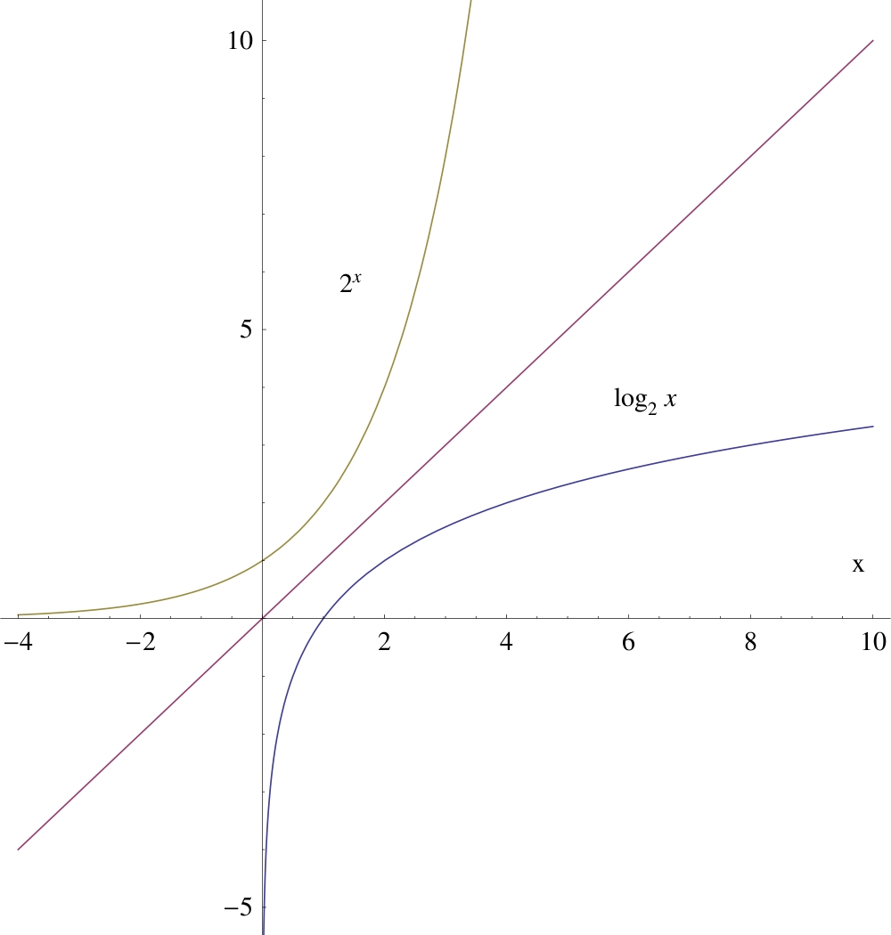
Note: The running time of any of the "fast" versions is not O(n) because n is not a measure of the size of n. The lg n is! (To be exact, size(n) = floor(log_2 n) + 1, or anything roughly proportional to it.)

Hence, the said running time is O(a^size(n)), where a > 1, that is, it is exponential.


Ackerman's function:

http://csc.csudh.edu/suchenek/CSC401/Ackermann3arg.java


Optimal BST


Number of binary search trees with n keys:

http://csc.csudh.edu/suchenek/CSC401/Mathematica/Number_of_all_BST_with_n_keys_etc.nb


Derivation of formula for A[ i ][ j ]


http://csc.csudh.edu/suchenek/CSC401/OptimalBSTrelation.pdf


Development of optimal BST program:


http://csc.csudh.edu/suchenek/CSC401/OPT_BST_rec.J


and its running time:

http://csc.csudh.edu/suchenek/CSC401/Mathematica/Analysis_of_recursive_building_opt_BST.nb


Development of optimal BST program (cont'd):


http://csc.csudh.edu/suchenek/CSC401/OPT_BST_dyn.J

http://csc.csudh.edu/suchenek/CSC401/OPT_BST_dyn_void.J


Sequence of computation of dynamic array:

http://csc.csudh.edu/suchenek/CSC401/Slides/Array_front_dynamic.pdf


Development of optimal BST program (cont'd):

http://csc.csudh.edu/suchenek/CSC401/OPT_BST_dyn_void_nonrec.J

http://csc.csudh.edu/suchenek/CSC401/OPT_BST.J

and computation of its running time:

http://csc.csudh.edu/suchenek/CSC401/Mathematica/OptBST_time.nb


Chapter 13 NP-Complete Problems

Readings:
Sections 13.1 - 13.3 and 13.7.1.


Fibonacci function "fast" implementation (see notes for chapter Dynamic Programming, "fast" Java implementation of the Fibonacci function) performs
O(a^size(n)) operations, where a > 1, that is, it is, it has an exponential  running time.

But Fibonacci function's recursive definition has this analytic solution


that can be computed in O((log n)^k), that is, O(size(n)^k), for some constant k. In particular, it can be computed in polynomial time in the worst case.

Can we accomplish that for all other problems that run in exponential time in the worst case?

For NP-complete problems (definition will be given, later) we don't know.


(Note. The Primality Test was once suspected NP-complete but now we know a program, invented by AKS, that solves it in O((log n)^k) (polynomial, that is) time.)

Link to slides

The following slides are copyrighted material, so the students in this class, and only the students in this class, are allowed to view these slides but not to copy or distribute them.

http://csc.csudh.edu/suchenek/CSC401/Slides/NP-complete_problems.pdf


Corrected definition of non-deterministic solution:

http://csc.csudh.edu/suchenek/CSC401/NondeterministicSolution.doc


Note.
If, rather than considering worst-case running time, we focus only on the average-case running time then some NP-complete problems become deterministically solvable in linear time (on average). Below is a link to a paper I wrote around 1988 which demonstrated that the CNF satisfiability problem is solvable in linear (with constant 2) time on average, under any reasonable comprehension of the adjective average. It is a result of the fact that most of Boolean functions on n variables must necessarily have exponentially-long (in n) propositional representations. (This observation has been attributed to Claude Shannon and is often referred to as Shannon's counting argument.) In other words, although deciding whether given CNF formula on n variables may require exponential (in n) running time, the lengths of vast majority of the shortest CNF formulas of n variables are also exponential (in n), thus making the average running time for such decision program linear in the size of its input.

Here is the link to my paper:

Technical Notes on Complexity of the Satisfiability Problem
http://arxiv.org/abs/1504.01092

Here is a link to a short and easy-to-read article in Communications of the ACM that lists some major positive developments in solving instances of CNF satisfiablity and practical implications thereof:

On P, NP, and Computational Complexity
https://cacm.acm.org/magazines/2010/11/100641-on-p-np-and-computational-complexity/fulltext


That's all, folks.


 Please, contact me right away if you have any questions.


Copyright © 2018 Suchenek - All rights reserved